How to turn a 1000-line messy SQL into a modular, & easy-to-maintain data pipeline?

• 1. Introduction
• 2. Split your SQL into smaller parts
  • 2.1. Start with a baseline validation to ensure that your changes do not change the output too much
  • 2.2. Split your CTAs/Subquery into separate functions (or models if using dbt)
  • 2.3. Unit test your functions for maintainability and evolution of logic
• 3. Conclusion
• 4. Required reading

1. Introduction

If you’ve been in the data space long enough, you would have come across really long SQL scripts that someone had written years ago. However, no one dares to touch them, as they may be powering some important part of the data pipeline, and everyone is scared of accidentally breaking them.

If you feel

Rough SQL is a good place to start, but it cannot scale after a certain limit

That dogmatic KISS approach leads to unmaintainable systems

The simplest solution that takes the shortest time is not always the most optimal.

The need to build the 80% solution and then rebuild the entire thing again if you need the 100% solution later is not better than creating the 100% solution so you don’t have to make it twice

Then this post is for you!

Imagine working with pipelines that are a joy to work with; any updates will be quick and straightforward.

In this post, we will see how to convert 1000-ish lines of messy SQL into modular code that is easy to test and modify. By the end of this post, you will have a systematic approach to converting your messy SQL queries into modular, well-scoped, easily testable code.

2. Split your SQL into smaller parts

Note: Code available at modular_code on GitHub.

2.1. Start with a baseline validation to ensure that your changes do not change the output too much

Before refactoring any code, it’s a good idea to form a test plan. When modularizing a long and messy SQL query, it’s best to create a single test that tests the entire query end-to-end.

Most of the time, the end-to-end tests on each refactor may not be possible due to the time it takes to run the query. In such cases, you can compare the data from the new code against the existing data (if you are refactoring a query, save the output into a table).

You can use tools like datacompy to compare existing data with data from the new code.

We use datacompy to keep track of differences in data from our mess sql and new modular code as shown here compare_dataset.py

Run datacompy as shown below:

> python compare_data.py
DataComPy Comparison
--------------------

DataFrame Summary
-----------------

  DataFrame  Columns  Rows
0       df1        7     6
1       df2        7     6

Column Summary
--------------

Number of columns in common: 7
Number of columns in df1 but not in df2: 0 []
Number of columns in df2 but not in df1: 0 []

Row Summary
-----------

Matched on: month, product_name, region_name
Any duplicates on match values: No
Absolute Tolerance: 0
Relative Tolerance: 0
Number of rows in common: 6
Number of rows in df1 but not in df2: 0
Number of rows in df2 but not in df1: 0

Number of rows with some compared columns unequal: 0
Number of rows with all compared columns equal: 6

Column Comparison
-----------------

Number of columns compared with some values unequal: 0
Number of columns compared with all values equal: 7
Total number of values which compare unequal: 0

Columns with Unequal Values or Types
------------------------------------

       Column df1 dtype df2 dtype  # Unequal  Max Diff  # Null Diff
0  sales_rank     int64    uint32          0       0.0            0

Sample Rows with Unequal Values
-------------------------------

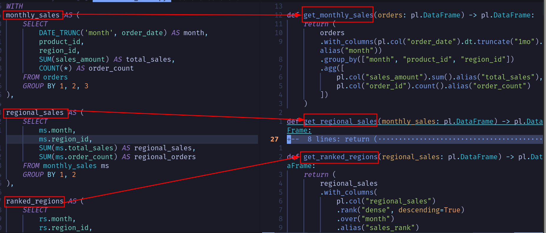
2.2. Split your CTAs/Subquery into separate functions (or models if using dbt)

It’s time to modularize your code. Isolate each CTA or subquery into a separate Python function (or dbt model). Name each function get_CTA_NAME(input_args), with input_args as the list of tables used for that CTA.

Each function should accept dataframes as inputs and return a dataframe as the output. Additionally, define the output schema for each Python function, enabling you to keep track of the columns.

Let’s see how this would look in our code:

Now that each CTA/Subquery is an individual function, you can link them together to create the final output .

if __name__ == "__main__":
    db_path = "database.db"
    orders, products, regions = read_base_tables(db_path)
    
    monthly_sales = get_monthly_sales(orders)
    regional_sales = get_regional_sales(monthly_sales)
    ranked_regions = get_ranked_regions(regional_sales)
    product_sales = get_product_sales(monthly_sales, products)
    final_result = get_final_result(product_sales, ranked_regions, regions)
    print(
      final_result
        .select(
          pl.col("month"),
          pl.col("product_name"),
          pl.col("category"), 
          pl.col("region_name"), 
          pl.col("product_sales"), 
          pl.col("regional_sales").alias("region_total_sales"), 
          pl.col("sales_rank")
        )
      )

Note that we are separating IO (reading from inputs and writing to outputs) from the data transformation. This is crucial to keeping the functions testable and ensuring that we can read/write from any environment as needed.

Read this link for more details on why to keep IO separate from data processing code .

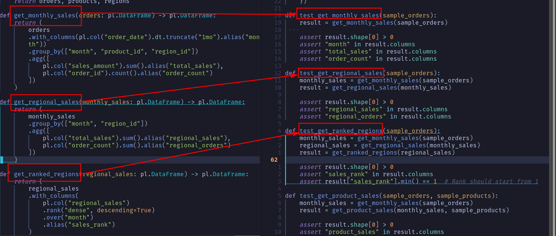
2.3. Unit test your functions for maintainability and evolution of logic

You can now create unit tests for individual functions. Unit tests ensure that your colleagues(and future self) have an idea of what the function is doing and are able to confidently make updates to the code without the fear of breaking something.

We can quickly add some tests (test_modular_code ) as shown below:

Read this post on how to use pytest effectively .

3. Conclusion

To recap, we saw how to split a 1000-line messy SQL query by

1. Creating a validation script to use throughout your modularization process
2. Splitting individual CTAs (or sub-query) into individual functions
3. Ensuring each function has test coverage for maintainability

The next time you are faced with a 1000-line nightmarish SQL query, follow the above steps to turn it into an easy-to-maintain modular code.

Please let me know in the comment section below if you have any questions or comments.

4. Required reading

1. Unit tests
2. Testing with pytest

If you found this article helpful, share it with a friend or colleague using one of the socials below!